> ## Documentation Index
> Fetch the complete documentation index at: https://docs.honeycomb.io/llms.txt
> Use this file to discover all available pages before exploring further.
# Visualize Concurrency
> Use the CONCURRENCY aggregate to chart how many spans are running at any given moment and spot resource contention in your system.
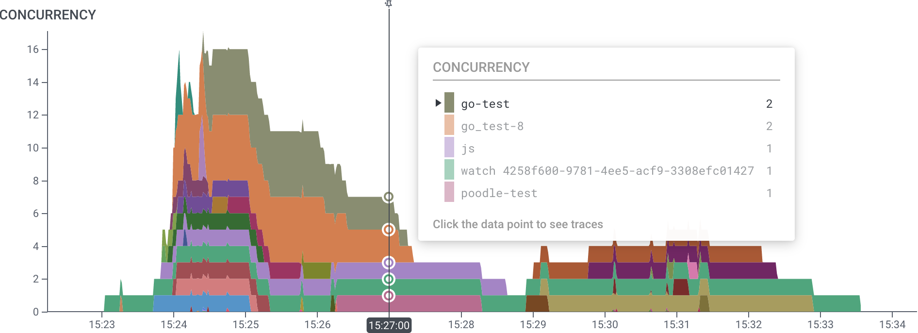
The `CONCURRENCY` aggregate [in a query](/investigate/query/build/) allows you to visualize how many spans are running at a given time.
It uses each span's duration to compute the fraction of each time interval covered by spans, extending right along the time axis.
This visualization can be useful to understand how much work a single resource is doing, or to understand the degree of overlap between independent traces.
The dataset must have a Span Duration field set in [Dataset Definitions](/configure/datasets/definitions/).
All tracing datasets have a Span Duration field set.
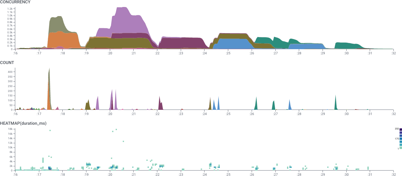
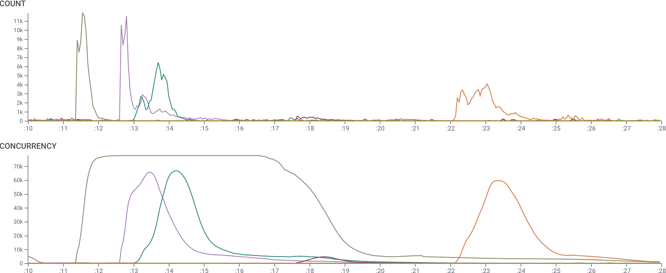
The following example is a graph of several concurrent traces generated by Honeycomb's storage engine.
Each span represents a single OS process.
Here, we have grouped by `trace.trace_id`, so each color bar is a distinct trace, but the number of processes involved in each varies.
The `CONCURRENCY` graph shows which traces are using the most resources, when, and to what extent they overlap.
Its y-axis shows the number of processes running at each moment.
In contrast, the `COUNT` aggregate below can only show what time each request started, neglecting its duration.
The `HEATMAP` aggregate can show duration, but not per trace.
It is very difficult to interpret the same information is via the `COUNT` and `HEATMAP` aggregates below.
 ## Conceptual Model of Concurrency
The `CONCURRENCY` aggregate counts the number of span that happen within each time interval.
A span counts toward the concurrency value if any part of it is in the interval.
Spans are counted fractionally: if the span is 50% in a segment, it counts as 0.5 toward the aggregate.
As an example, consider the set of spans shown in the figure below.
Each span has a start time and a duration. The top span, for instance, has a start time of :00 and a duration of 3 seconds.
## Conceptual Model of Concurrency
The `CONCURRENCY` aggregate counts the number of span that happen within each time interval.
A span counts toward the concurrency value if any part of it is in the interval.
Spans are counted fractionally: if the span is 50% in a segment, it counts as 0.5 toward the aggregate.
As an example, consider the set of spans shown in the figure below.
Each span has a start time and a duration. The top span, for instance, has a start time of :00 and a duration of 3 seconds.
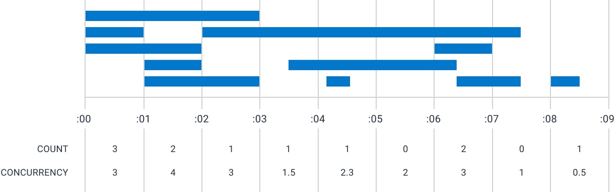 The `COUNT` operator counts only the number of events that start within this time period.
The :00 time period starts three events, while the :01 period starts two events.
The `CONCURRENCY` operator counts all events that cross through the time period: three for :00, but four for :01.
It is important to note that the `CONCURRENCY` aggregate is an estimate rather than a full-resolution graph of actual span concurrency.
It creates this estimate by summing how much of each time bucket is covered by each span.
If your query has 1-minute granularity, 60 1-second spans appearing in a single minute (whether they overlap or not) will each contribute 1/60 of a count -- and so would yield a `CONCURRENCY` of 1.
A single 60-second span in the same minute would also yield a `CONCURRENCY` of 1.
This estimation is most accurate with fine granularity, so in most cases `CONCURRENCY` is most useful when highly zoomed into a narrow time range.
To properly account for spans which begin before the query time range, `CONCURRENCY` looks for spans beginning a full hour before the start of the query.
Spans with duration greater than one hour are not counted if they begin more than an hour before query start.
The result table for `CONCURRENCY` shows the highest value of concurrency in that series.
It is worth emphasizing that `CONCURRENCY` works differently from other Honeycomb aggregates.
All other operators pin their data to the span start time.
A `COUNT` or `AVG` only examines the value at the time that the span starts.
In contrast, `CONCURRENCY` fills in values through the entire duration of the span.
## Use Cases for the CONCURRENCY Aggregate
The `CONCURRENCY` aggregate can be used in a number of different ways.
### Resource Contention
The most common use is to measure resource contention -- it can help show how many things are using a single resource at a given time.
For example, if a system implements a queue, you could instrument it so that a span represents time waiting on the queue.
The `CONCURRENCY` aggregate would then show the queue depth at any point -- the number of spans still in the queue.
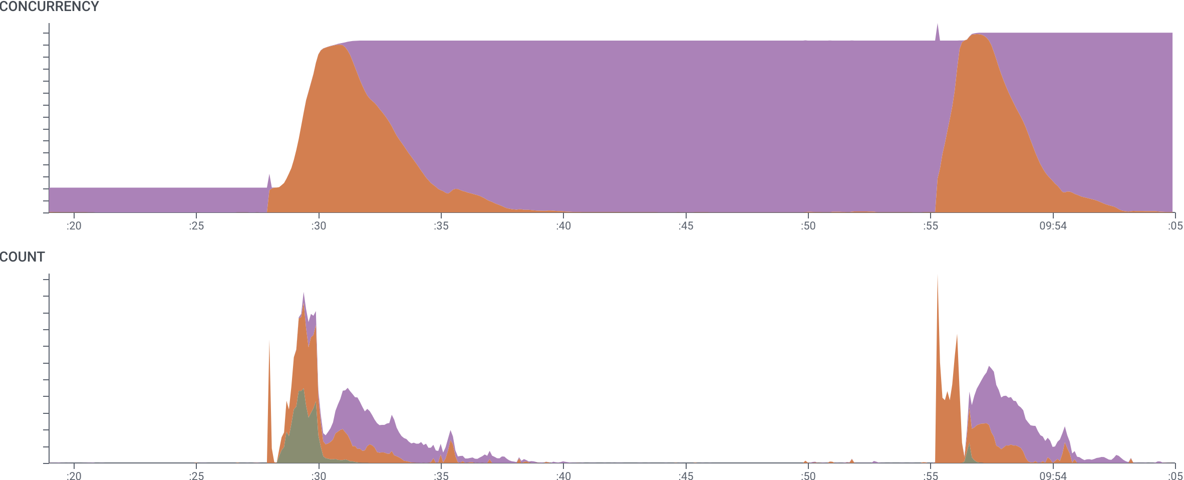
Here, we show a dataset where resources can change between states: they `start` (green), and then either `run` (orange), or `sleep` (purple).
Querying `CONCURRENCY`, grouped by state, allows us to see how many of the resource we have in each state.
`Start` spans have very short duration and so are only visible in the `COUNT` graph, but the alternating `run` and `sleep` groups in `CONCURRENCY` represents the demand curve and level of idle capacity.
(The y-axis labels are redacted.)
The `COUNT` operator counts only the number of events that start within this time period.
The :00 time period starts three events, while the :01 period starts two events.
The `CONCURRENCY` operator counts all events that cross through the time period: three for :00, but four for :01.
It is important to note that the `CONCURRENCY` aggregate is an estimate rather than a full-resolution graph of actual span concurrency.
It creates this estimate by summing how much of each time bucket is covered by each span.
If your query has 1-minute granularity, 60 1-second spans appearing in a single minute (whether they overlap or not) will each contribute 1/60 of a count -- and so would yield a `CONCURRENCY` of 1.
A single 60-second span in the same minute would also yield a `CONCURRENCY` of 1.
This estimation is most accurate with fine granularity, so in most cases `CONCURRENCY` is most useful when highly zoomed into a narrow time range.
To properly account for spans which begin before the query time range, `CONCURRENCY` looks for spans beginning a full hour before the start of the query.
Spans with duration greater than one hour are not counted if they begin more than an hour before query start.
The result table for `CONCURRENCY` shows the highest value of concurrency in that series.
It is worth emphasizing that `CONCURRENCY` works differently from other Honeycomb aggregates.
All other operators pin their data to the span start time.
A `COUNT` or `AVG` only examines the value at the time that the span starts.
In contrast, `CONCURRENCY` fills in values through the entire duration of the span.
## Use Cases for the CONCURRENCY Aggregate
The `CONCURRENCY` aggregate can be used in a number of different ways.
### Resource Contention
The most common use is to measure resource contention -- it can help show how many things are using a single resource at a given time.
For example, if a system implements a queue, you could instrument it so that a span represents time waiting on the queue.
The `CONCURRENCY` aggregate would then show the queue depth at any point -- the number of spans still in the queue.
Here, we show a dataset where resources can change between states: they `start` (green), and then either `run` (orange), or `sleep` (purple).
Querying `CONCURRENCY`, grouped by state, allows us to see how many of the resource we have in each state.
`Start` spans have very short duration and so are only visible in the `COUNT` graph, but the alternating `run` and `sleep` groups in `CONCURRENCY` represents the demand curve and level of idle capacity.
(The y-axis labels are redacted.)
 ### Trace Depth
Another use of a `CONCURRENCY` aggregate is to show the depth of multiple traces.
In this example, we are examining a system that starts massively-parallel compute jobs.
We have grouped by `trace.trace_id`, so this query shows how many spans are operative at a time in each trace.
The curve shows that while several traces had many spans, one trace in particular utilized many more resources for a much longer time than the others.
### Trace Depth
Another use of a `CONCURRENCY` aggregate is to show the depth of multiple traces.
In this example, we are examining a system that starts massively-parallel compute jobs.
We have grouped by `trace.trace_id`, so this query shows how many spans are operative at a time in each trace.
The curve shows that while several traces had many spans, one trace in particular utilized many more resources for a much longer time than the others.
 ### Trace Summary
A third use of the aggregate is to look at a single trace and break down its internal processes.
In this image, we have selected a single trace of our build process, grouped by `name`.
This view of `CONCURRENCY` gives a succinct visualization of the trace that shows how many spans of each type were active at each time.
### Trace Summary
A third use of the aggregate is to look at a single trace and break down its internal processes.
In this image, we have selected a single trace of our build process, grouped by `name`.
This view of `CONCURRENCY` gives a succinct visualization of the trace that shows how many spans of each type were active at each time.