> ## Documentation Index
> Fetch the complete documentation index at: https://docs.honeycomb.io/llms.txt
> Use this file to discover all available pages before exploring further.
# Build a Query
> Construct queries against your telemetry data using Query Builder. Add filters, breakdowns, and calculations manually or start from a natural language prompt.
export const FlexStyleTable = ({columns, overflowWrap = "normal", children}) => {
const colWidths = columns ? columns.trim().split(/\s+/) : [];
const scopeKey = [columns || "auto", overflowWrap].join("-").replace(/[^a-zA-Z0-9-]/g, "-");
const colRules = colWidths.map((width, i) => `[data-fst="${scopeKey}"] table th:nth-of-type(${i + 1}) { width: ${width}; }`).join("\n");
const css = `
[data-fst="${scopeKey}"] table {
table-layout: ${colWidths.length > 0 ? "fixed" : "auto"};
width: 100%;
}
${colRules}
[data-fst="${scopeKey}"] table td { overflow-wrap: ${overflowWrap}; }
`.trim();
return
{children}
;
};
export const SchemaTable = ({children}) => {
return
{children}
;
};
export const HnyIcon = ({alias, path, size = 16, iconColor}) => {
const iconMap = {
"home": "house.svg",
"marker": "caretFilledDown.svg",
"show-marker-options": "chatTextLeft.svg",
"download": "arrowLineDown.svg",
"trace-waterfall": "trace.svg",
"show-query-details": "listDashes.svg",
"table": "table.svg",
"log-lines": "logLines.svg",
"chart": "chartLine.svg",
"show-settings": "gear.svg",
"add": "plus.svg",
"remove": "delete.svg",
"persist": "caretDown.svg",
"close": "close.svg",
"copy": "copy.svg",
"zoom-in": "magnifyingGlassPlus.svg",
"zoom-out": "magnifyingGlassMinus.svg",
"color-assignment": "drop.svg",
"drag": "dots-six-vertical.svg",
"drawer": "drawer.svg",
"show-actions": "dotsThree.svg",
"edit": "pencil.svg",
"delete": "trash.svg",
"move": "arrowsOutCardinal.svg",
"show-legend": "circleInfo.svg",
"usage-ok": "usageGood.svg",
"usage-warning": "usageWarning.svg",
"usage-danger": "usageDanger.svg",
"open-query-builder": "query.svg",
"home-menu": "house.svg",
"query-menu": "query.svg",
"boards-menu": "board.svg",
"triggers-menu": "bell.svg",
"slos-menu": "handshake.svg",
"service-map-menu": "serviceMap.svg",
"history-menu": "clockCounterClockwise.svg",
"manage-data-menu": "cube.svg",
"usage-menu": "usageGood.svg",
"canvas-menu": "sparkle.svg",
"anomalies-menu": "anomalies.svg",
"show-details": "dotsThreeVertical.svg",
"resize-handle": "board-panel-resize-handle.png",
"standard-dataset": "cube.svg",
"trace-dataset": "cubeChat.svg",
"all-datasets": "linkedSquares.svg",
"share": "arrowBentRight.svg",
"run-in-query-builder": "arrowSquareUpRight.svg",
"link": "link.svg",
"text": "text.svg",
"receive": "arrowLineDown.svg",
"process": "lightning.svg",
"sample": "drop.svg",
"send": "arrowLineUp.svg",
"submit": "arrowUp.svg",
"canvas-menu": "sparkle.svg",
"canvas": "sparkle.svg",
"chat-about-this-page": "sparkle.svg",
"private": "lockKey.svg",
"shared": "people.svg",
"expand": "caretDown.svg",
"previous": "caretLeft.svg",
"next": "caretRight.svg",
"expand-chat": "caretLeft.svg",
"minimize-chat": "caretRight.svg",
"open-in-canvas": "arrowSquareUpRight.svg"
};
const iconBasePath = "/_assets/icons/";
const iconPath = path || (alias ? `${iconBasePath}${iconMap[alias]}` : undefined);
return ;
};
**Query Builder** allows you to construct queries against your data to produce results for investigation and further exploration.
With Query Builder, enter field names, operators, and/or field values in clauses to construct or modify a query.
Use Query Builder to explore your data.
## Accessing Query Builder
In the left navigation menu, select **Query** ().
When the left navigation menu is compact, only the Query menu icon appears.
## Interacting with Query Builder
Below is an example of a blank Query Builder.
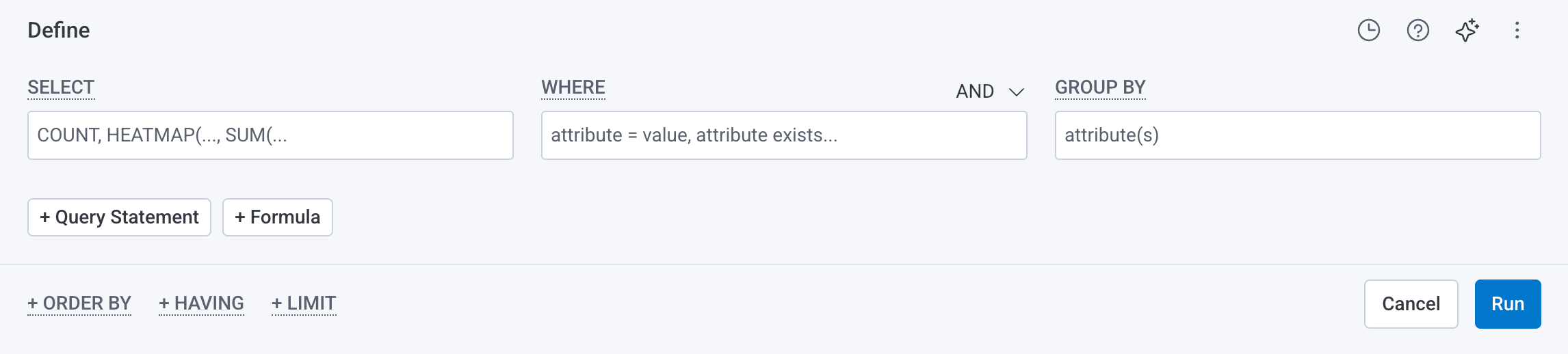 Generate Honeycomb queries using natural language with [Query Assistant](/investigate/query/build/query-assistant).
### Clauses
A query in Honeycomb consists of up to six clauses:
* [**SELECT**](#visualize) - Performs a calculation and displays a corresponding graph over time. Most **SELECT** queries return a line graph while the `HEATMAP` visualization shows the distribution of data over time
* [**WHERE**](#where) - Filters based on field or attribute parameter(s)
* [**GROUP BY**](#group-by) - Groups fields by field or attribute parameter(s)
* [**ORDER BY**](#order-by) - Sort the results
* [**LIMIT**](#limit) - Specify a limit on how many results to return
* [**HAVING**](#having) - Filter results based on aggregate criteria
### Relational Fields
You can use relational fields in the **WHERE** and **GROUP BY** clauses to narrow your query to find traces that contain fields and values within a specific span type.
You can identify span types by their prefix.
Relational fields are available for use only within the Query Builder in the Honeycomb UI and only within the **WHERE** and **GROUP BY** clauses.
Using relational fields automatically applies **AND** operators to the containing clause; all conditions within the clause must be met.
#### Prefixes
Relational field span prefixes follow your trace structure and include:
* `root.` - Matches to the root span within a trace. Any additional filters in your query will search through fields only in the matched `root.` span.
* `parent.` - Matches to a direct parent span within a trace. Any additional filters in your query will search through fields only in the specified `parent.` span and its immediate child spans.
* `child.` - Matches to a single child span within a trace and returns the corresponding parent span. Any additional filters in your query will search through fields only in the matched `child.` span.
* `anyX.` (`any.`, `any2.`, `any3.`) - Matches to a single span anywhere in the trace. Use `anyX.` prefixes together to query for a trace that contains up to three spans, each with their own filters. Any additional filters applied to the same `anyX.` prefix will apply to the same matched span.
* `none.` - Matches to a single span and excludes any traces that contain that matched span. Any additional filters in your query will search through only fields not in the matched `none.` span.
Using multiple of the same `anyX.` prefix will find many fields on a single span.
Using an `anyX.` prefix in a **GROUP BY** clause requires specifying a field.
## Using Query Builder
To use Query Builder, enter terms.
For examples to try, refer to our [Query Examples](/investigate/query/examples-traces/).
As you type, Honeycomb autocomplete prompts with [relational field prefixes](#prefixes) and selectable query components.
Execute the query by selecting **Run Query** or pressing Shift + Enter on the keyboard.
Honeycomb supports keyboard shortcuts!
Refer to a list of supported actions by typing `?` while on the Query Builder page.
### Using Relational Fields
When you apply relational fields to your query, you can extend queries to use qualifying relationships that indicate where and how spans appear in a trace.
For example, if you managed an e-commerce platform and were trying to determine how many users received an error when they applied a discount code during checkout, you would be interested in finding any applicable spans in your trace.
This example query uses both the `root.` and `anyX.` prefixes to find the count of all spans where an error exists, where any span in the same trace is named `getDiscounts` and where its root span is named `/cart/checkout`.
| CLAUSE | VALUE | DESCRIPTION |
| -------- | ------------------------------------------------------------------------------------------- | -------------------------------------------------------------------------------------------------------------------------------------------------------------------------------------------------------------------------------------------------------------------------------------- |
| SELECT | COUNT | Calculates count. |
| WHERE | `error exists` AND
Generate Honeycomb queries using natural language with [Query Assistant](/investigate/query/build/query-assistant).
### Clauses
A query in Honeycomb consists of up to six clauses:
* [**SELECT**](#visualize) - Performs a calculation and displays a corresponding graph over time. Most **SELECT** queries return a line graph while the `HEATMAP` visualization shows the distribution of data over time
* [**WHERE**](#where) - Filters based on field or attribute parameter(s)
* [**GROUP BY**](#group-by) - Groups fields by field or attribute parameter(s)
* [**ORDER BY**](#order-by) - Sort the results
* [**LIMIT**](#limit) - Specify a limit on how many results to return
* [**HAVING**](#having) - Filter results based on aggregate criteria
### Relational Fields
You can use relational fields in the **WHERE** and **GROUP BY** clauses to narrow your query to find traces that contain fields and values within a specific span type.
You can identify span types by their prefix.
Relational fields are available for use only within the Query Builder in the Honeycomb UI and only within the **WHERE** and **GROUP BY** clauses.
Using relational fields automatically applies **AND** operators to the containing clause; all conditions within the clause must be met.
#### Prefixes
Relational field span prefixes follow your trace structure and include:
* `root.` - Matches to the root span within a trace. Any additional filters in your query will search through fields only in the matched `root.` span.
* `parent.` - Matches to a direct parent span within a trace. Any additional filters in your query will search through fields only in the specified `parent.` span and its immediate child spans.
* `child.` - Matches to a single child span within a trace and returns the corresponding parent span. Any additional filters in your query will search through fields only in the matched `child.` span.
* `anyX.` (`any.`, `any2.`, `any3.`) - Matches to a single span anywhere in the trace. Use `anyX.` prefixes together to query for a trace that contains up to three spans, each with their own filters. Any additional filters applied to the same `anyX.` prefix will apply to the same matched span.
* `none.` - Matches to a single span and excludes any traces that contain that matched span. Any additional filters in your query will search through only fields not in the matched `none.` span.
Using multiple of the same `anyX.` prefix will find many fields on a single span.
Using an `anyX.` prefix in a **GROUP BY** clause requires specifying a field.
## Using Query Builder
To use Query Builder, enter terms.
For examples to try, refer to our [Query Examples](/investigate/query/examples-traces/).
As you type, Honeycomb autocomplete prompts with [relational field prefixes](#prefixes) and selectable query components.
Execute the query by selecting **Run Query** or pressing Shift + Enter on the keyboard.
Honeycomb supports keyboard shortcuts!
Refer to a list of supported actions by typing `?` while on the Query Builder page.
### Using Relational Fields
When you apply relational fields to your query, you can extend queries to use qualifying relationships that indicate where and how spans appear in a trace.
For example, if you managed an e-commerce platform and were trying to determine how many users received an error when they applied a discount code during checkout, you would be interested in finding any applicable spans in your trace.
This example query uses both the `root.` and `anyX.` prefixes to find the count of all spans where an error exists, where any span in the same trace is named `getDiscounts` and where its root span is named `/cart/checkout`.
| CLAUSE | VALUE | DESCRIPTION |
| -------- | ------------------------------------------------------------------------------------------- | -------------------------------------------------------------------------------------------------------------------------------------------------------------------------------------------------------------------------------------------------------------------------------------- |
| SELECT | COUNT | Calculates count. |
| WHERE | `error exists` AND
`any.name = getDiscounts` AND
`root.name = /cart/checkout` | Applies conditions to narrow your query: - An error exists (primary condition)
- The span is in the same trace and is named `getDiscounts` (secondary condition)
- The span is contained within a root span named `/cart/checkout/` (secondary condition)
|
| GROUP BY | `error` | Groups by the error. |
After querying, you might see the following trace summary when you select a span from the query results:
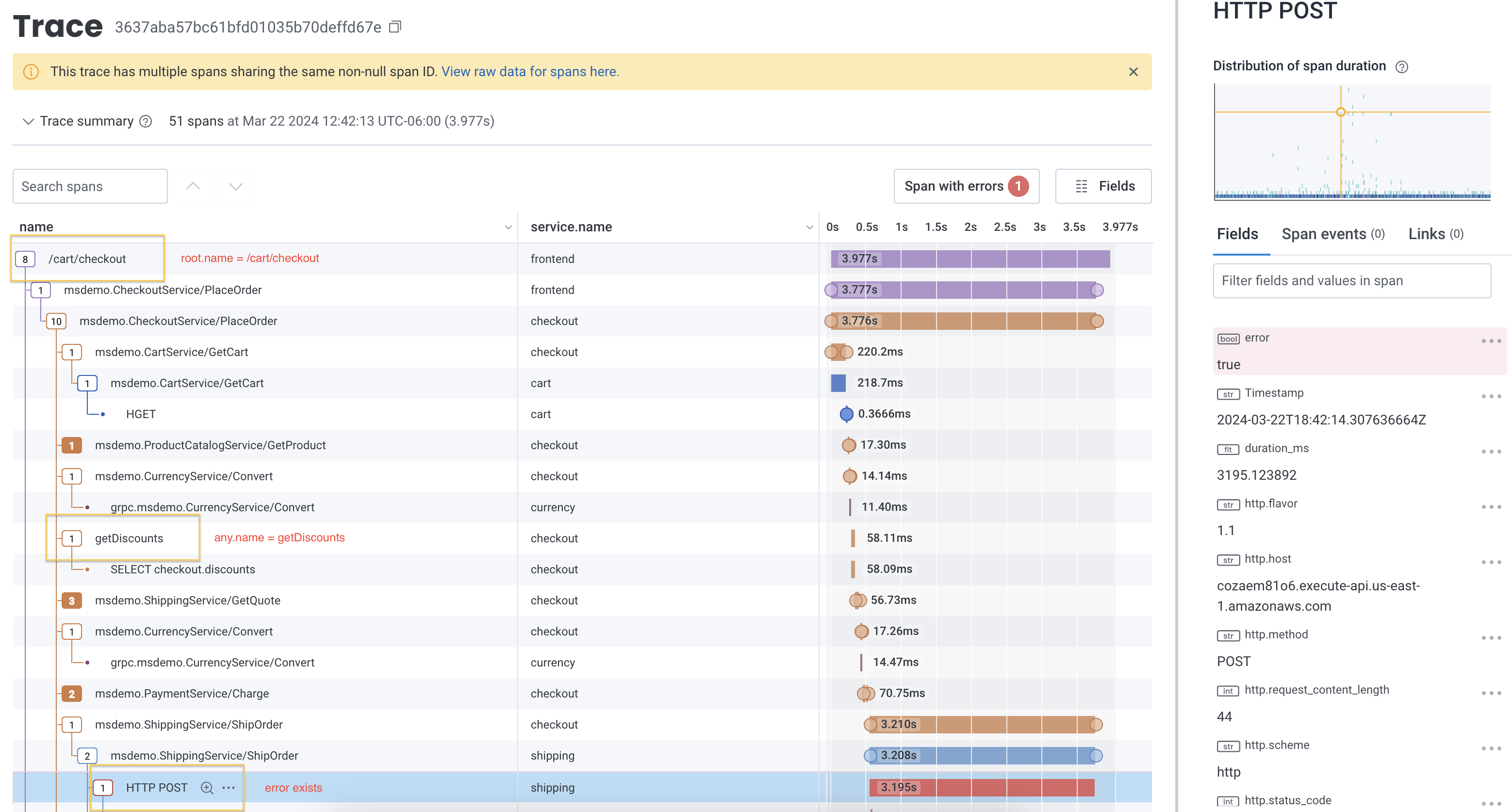 To learn more about how to use relational fields with specific span types, visit [Query Reference: Relational Fields](#relational-fields-1).
## Query Builder Results
The default output for most queries will include:
1. a visualization, or a graph over time
2. a [summary table](#select-summary-table)
The precise composition depends on what your query contains.
* Specifying a **SELECT** clause causes a visualization to be drawn, representing that calculated value over time
* Multiple **SELECT** clauses result in multiple graphs, one for each calculation.
* Specifying a **GROUP BY** clause results in the graph having multiple lines, one for each group.
The summary table will contain a single row for each unique group.
* Leaving **SELECT** blank results in raw event data being returned without any summarization.
## Editing Queries in Query Builder
Click on any box in the Query Builder to edit the clauses there.
Selecting the **X** removes the field from the clause.
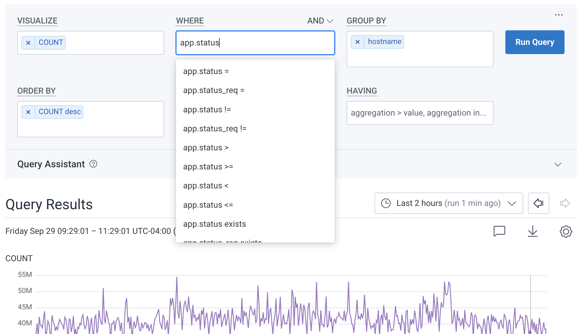
In the image below, the user already entered **SELECT** `COUNT` and **GROUP BY** `hostname`.
When editing, they add a new **WHERE** clause on `app.status_code`.
Honeycomb autocomplete helps construct the query.
To learn more about how to use relational fields with specific span types, visit [Query Reference: Relational Fields](#relational-fields-1).
## Query Builder Results
The default output for most queries will include:
1. a visualization, or a graph over time
2. a [summary table](#select-summary-table)
The precise composition depends on what your query contains.
* Specifying a **SELECT** clause causes a visualization to be drawn, representing that calculated value over time
* Multiple **SELECT** clauses result in multiple graphs, one for each calculation.
* Specifying a **GROUP BY** clause results in the graph having multiple lines, one for each group.
The summary table will contain a single row for each unique group.
* Leaving **SELECT** blank results in raw event data being returned without any summarization.
## Editing Queries in Query Builder
Click on any box in the Query Builder to edit the clauses there.
Selecting the **X** removes the field from the clause.
In the image below, the user already entered **SELECT** `COUNT` and **GROUP BY** `hostname`.
When editing, they add a new **WHERE** clause on `app.status_code`.
Honeycomb autocomplete helps construct the query.
 ### Change Datasets
In the upper left corner above the Query Builder, use the **Dataset Switcher** to choose to query a specific Dataset or all Datasets within your Environment.
The latter option may be useful if you need to reference events that span across multiple services.
When you switch datasets, Honeycomb will load the existing query on that dataset, but it will not run it automatically.
You can also set a default scope for new queries per environment in [Environment Settings](/reference/honeycomb-ui/environment/environment-settings/).
### Change and Compare Query Time Ranges
In the bottom right corner below the Query Builder, use the **time picker** to modify the selected time span of the data in your query.
Use a preset time range or a custom time range.
Honeycomb supports running queries across different periods of time, so you can compare results to see how your systems change.
Run a Time Comparison query by selecting a time range under **Compare to previous time period** in the time picker.
Honeycomb then will run a query as defined in the Query Builder and another query for the time comparison range selected.
## Query Reference
### SELECT
Honeycomb supports a wide range of calculations to provide insight into your events.
When a grouping is provided, calculations occur within each group; otherwise, anything calculated is done so over all matching events.
For example, say you have collected the following events from your web server logs:
| Timestamp | uri | status\_code | response\_time\_ms |
| :--------------- | :----- | :----------- | :----------------- |
| 2016-08-01 07:30 | /about | 500 | 126 |
| 2016-08-01 07:45 | /about | 200 | 57 |
| 2016-08-01 07:57 | /docs | 200 | 82 |
| 2016-08-01 08:03 | /docs | 200 | 23 |
Specifying a visualization for a particular attribute (`P95(response_time_ms)`for example) means to apply the aggregation function (in this case, `P95`, or taking the 95th [percentile](https://en.wikipedia.org/wiki/Percentile)) over the values for the attribute (`response_time_ms`) across all input events.
Defining multiple **SELECT** clauses is common and can be useful, especially when comparing their outputs to each other.
For example, it can be useful to see both the `COUNT` and the `P95(duration)` for a set of events to understand whether latency changes follow volume changes.
While most **SELECT** queries return a line graph, the [`HEATMAP`](/investigate/analyze/visualize-events/) visualization allows you see the distribution of data in a rich and interactive way.
Heatmaps also allow you to find outliers in data using [BubbleUp](/investigate/analyze/identify-outliers/).
#### SELECT: Basic Case
Scenario: we want to capture overall statistics for our web server.
Given our four-event dataset [described above](#select), consider a query which contains:
* Visualize the overall `COUNT`
* Visualize the `AVG` of `response_time_ms` values
* Visualize the `P95` of `response_time_ms` values
These calculations would return statistics across the entirety of our dataset:
| COUNT | AVG(response\_time\_ms) | P95(response\_time\_ms) |
| :---- | :---------------------- | :---------------------- |
| 4 | 72 | 119.4 |
#### SELECT: COUNT\_DATAPOINTS
`COUNT_DATAPOINTS` returns the total count of datapoints ingested across all metric fields in a metrics dataset. Use it to understand data volume and track what is driving your usage. The `COUNT_DATAPOINTS` aggregate can only be used with time-series metrics data.
A **datapoint** is a single recorded value for a metric at a point in time, for a unique combination of attributes. Datapoints are the unit by which metrics usage is billed. Every active time series is a unique combination of metric name and attributes, such as `http.server.request.duration` where `k8s.node.name=node-1` which continuously produces datapoints over time. High attribute cardinality means more time series, and therefore more datapoints.
Use `COUNT_DATAPOINTS` to track billing usage over a time range or to spot metric ingestion spikes.
`COUNT_DATAPOINTS` data is only available from February 13, 2026 onward. Queries that include time ranges before this date will only reflect data ingested after that date.
#### SELECT: COUNT\_DATAPOINTS(metric\_field\_name)
`COUNT_DATAPOINTS()` returns the count of datapoints for a specific metric field. Only rows where that column has a value are counted. The `COUNT_DATAPOINTS()` aggregate can only be used with time-series metrics data.
Use this when you want to isolate the datapoint volume of a single metric. For example, comparing ingestion across metrics or identifying which metric is driving a cost increase.
If any metric data has been deleted, `COUNT_DATAPOINTS` will still include those deleted datapoints in its count. `COUNT_DATAPOINTS(metric_field_name)` excludes deleted data.
### SELECT: HISTOGRAM\_COUNT(metric\_field\_name)
`HISTOGRAM_COUNT()` returns the count of observations in a histogram metric field, across the rows and time included in the query.
This aggregate can only be used on time series metrics histogram fields.
#### SELECT Summary Table
The **SELECT** clause returns both a time series graph and a column of values in the result summary table.
Note that in the graph, the values shown are aggregated for each interval at the current granularity.
Conversely, the values shown in the summary table are calculated across the entire time range for that query.
These results can be a little surprising for some calculations.
The `P95(duration_ms)` across the entire time range may not look quite like the `P95` value at any given point of the curve, because there may be spikes and bumps in the underlying data that are hidden in the time intervals.
The summary table for a `HEATMAP` shows a histogram of values of that field across the full time range.
#### SELECT Operations
Most **SELECT** operations take a single argument, with the exception of `COUNT` and `COUNT_DATAPOINTS`, that optionally take an argument, and `CONCURRENCY`, which takes no arguments.
Events that do not have a relevant attribute are ignored, and will not be counted in aggregations.
In the chart below, `` refers to any field name while the `` argument refers to a float or integer field.
| Aggregate | Meaning |
| ------------------------------------------------ | -------------------------------------------------------------------------------------------------------------------------------------------------------------------------------------------------------- |
| `COUNT` | The number of events |
| `COUNT()` | The number of events with a non-null value for a field |
| `COUNT_DISTINCT()` | The count of different distinct values in a field. `COUNT_DISTINCT` is estimated using the HyperLogLog algorithm. |
| `COUNT_DATAPOINTS` | The total count of datapoints ingested across all metric fields in a metrics dataset. |
| `COUNT_DATAPOINTS()` | The count of datapoints for a specified metric field in a metrics dataset. Only rows where the specified field has a value are counted. |
| `HISTOGRAM_COUNT()` | The count of observations recorded in a specified histogram field. Requires a histogram field in a time series metrics dataset as the parameter. |
| `SUM()` | The sum of the field value |
| `AVG()` | The average value of the field |
| `MAX()` | The maximum value of the field |
| `MIN()` | The minimum value of the field |
| `P001()` | The .1-th percentile of the field. `P001` is estimated using the t-digest algorithm. |
| `P01()` | The 1st percentile of the field. `P01` is estimated using the t-digest algorithm. |
| `P05()` | The 5th percentile of the field. `P05` is estimated using the t-digest algorithm. |
| `P10()` | The 10th percentile of the field. `P10` is estimated using the t-digest algorithm. |
| `P20()` | The 20th percentile of the field. `P20` is estimated using the t-digest algorithm. |
| `P25()` | The 25th percentile of the field. `P25` is estimated using the t-digest algorithm. |
| `P50()` | The 50th percentile of the field. `P50` is estimated using the t-digest algorithm. |
| `P75()` | The 75th percentile of the field. `P75` is estimated using the t-digest algorithm. |
| `P80()` | The 80th percentile of the field. `P80` is estimated using the t-digest algorithm. |
| `P90()` | The 90th percentile of the field. `P90` is estimated using the t-digest algorithm. |
| `P95()` | The 95th percentile of the field. `P95` is estimated using the t-digest algorithm. |
| `P99()` | The 99th percentile of the field. `P99` is estimated using the t-digest algorithm. |
| `P999()` | The 99.9th percentile of the field. `P999` is estimated using the t-digest algorithm. |
| `HEATMAP()` | A heatmap of the distribution of that field |
| `CONCURRENCY` | The concurrency of the current query, for tracing-enabled datasets only. This is a complex operation; please see the [detailed explanatory page](/investigate/query/build/visualize-concurrency/) on it. |
| `RATE_AVG()` | The difference between subsequent field values after applying the `RATE_AVG` operator. [Learn more about the RATE operators](/investigate/query/build/visualize-rate/). |
| `RATE_SUM()` | The difference between subsequent field values after applying the `RATE_SUM` operator. [Learn more about the RATE operators](/investigate/query/build/visualize-rate/). |
| `RATE_MAX()` | The difference between subsequent field values after applying the `RATE_MAX` operator. [Learn more about the RATE operators](/investigate/query/build/visualize-rate/). |
### WHERE
The **WHERE** clause allows you to constrain events by some attribute besides time. For example, you may want to ignore an outlier case or isolate events triggered by a particular actor or circumstance.
For example, say you have collected the following events from your web server logs:
| Timestamp | uri | status\_code |
| :--------------- | :----- | :----------- |
| 2016-08-01 08:15 | /about | 500 |
| 2016-08-01 08:22 | /about | 200 |
| 2016-08-01 08:27 | /docs | 403 |
You can define any number of arbitrary constraints based on event values.
**WHERE** clauses work in concert with the specified time range to define the events that are ultimately considered by any **GROUP BY** or **SELECT** clauses.
The **WHERE** clause does not require string delimiters or escape characters. For example, to match a URI of `/docs`, you can enter `uri = /docs`.
#### WHERE: Basic Case
Scenario: we want to understand the frequency of unsuccessful web requests.
Given our three-event dataset [described above](#where), consider a query which contains:
* **SELECT** the overall `COUNT`
* **WHERE** `status_code != 200`
The **WHERE** clause removes the successful event (our `/about` web request returning a `200`) from consideration, and only counts the first and third events towards our **SELECT** clause:
| COUNT |
| :---- |
| 2 |
#### WHERE: Multiple Clauses
Scenario: we want to refine our constraints further, to span multiple attributes for each event.
Combining **WHERE** clauses returns events that satisfy either the **intersection** of all specified **WHERE** clauses, or the **union**.
Given our three-event dataset [described above](#where), consider a query which contains:
* Where `uri = "/about"`
* AND `status_code != 200`
As all three events are considered by the **WHERE** clauses, only the first one satisfies both:
| Timestamp | uri | status\_code |
| :--------------- | :----- | :----------- |
| 2016-08-01 08:55 | /about | 500 |
Honeycomb also allows you to look at the **union** of clauses by setting to an `OR`.
* **WHERE** `status_code = 500`
* OR `status_code = 403`
| Timestamp | uri | status\_code |
| :--------------- | :----- | :----------- |
| 2016-08-01 08:55 | /about | 500 |
| 2016-08-01 08:27 | /docs | 403 |
#### WHERE: Relational Fields
You can use relational fields in your **WHERE** clause to narrow your query to find traces that contain fields and values within a specific span type.
To learn more and explore some examples, visit [Relational Fields](#relational-fields-1) in this reference.
#### WHERE Operations
`WHERE` operations may take one or more attributes.
Events are only counted if they have a relevant attribute, except in the case of the `does-not-exist` operation.
| Operation | Opposite | Arguments | Meaning |
| :------------ | :-------------------- | :-------- | :------------------------------------------------------------------------------ |
| `=` | `!=` | 1 | Exact numerical or string match |
| `starts-with` | `does-not-start-with` | 1 | String start match |
| `ends-with` | `does-not-end-with` | 1 | String end match |
| `exists` | `does-not-exist` | 0 | Checks for non-null values |
| `>`, `>=` | `<`, `<=` | 1 | numerical comparison |
| `contains` | `does-not-contain` | 1 | string inclusion: checks whether the attribute matches a substring of the value |
| `in` | `not-in` | 1+ | list inclusion: checks whether the attribute matches any item in the list |
The syntax for the `in` operator does not use parentheses.
For example, `request_method in GET,POST`
### GROUP BY
Being able to separate a series of events into groups by attribute is a powerful way to compare segments of your dataset against each other.
For example, say you have collected the following events from your web server logs:
| Timestamp | uri | status\_code |
| :--------------- | :----- | :----------- |
| 2016-08-01 07:30 | /about | 500 |
| 2016-08-01 07:45 | /about | 200 |
| 2016-08-01 07:57 | /docs | 200 |
You might want to analyze your web traffic in groups based on the `uri` ("/about" vs "/docs") or the `status_code` (`500` versus `200`).
Choosing to group by `uri` would return two result rows: one representing events in which `uri="/about"` and another representing events in which `uri="/docs"`.
Each of these grouped results rows will be represented by a single line on a graph.
When using GROUP BY for more than one attribute, Honeycomb will consider each unique combination of values as a single group.
Here, choosing to group by both `uri` and `status_code` will return three groups: `/about`+`500`, `/about`+`200`, and `/docs`+`200`.
Grouping, paired with calculation, can often reveal interesting patterns in your underlying events—grouping by `uri`, for example, and calculating response time stats will show you the slowest (or fastest) `uri`s.
Honeycomb supports grouping your data based on any attribute in an event, though you will likely receive the clearest results by choosing an attribute with an uneven distribution within your data.
The **GROUP BY** dropdown list also has a shortcut to [create a calculated field](/configure/environments/calculated-fields/).
#### Grouping and Selecting: Better Together
Scenario: we want to examine performance of our web server by endpoint.
Given our four-event dataset [described above](#select), consider a query which contains:
* Group by `uri`
* Select the overall `COUNT`
* Select the `AVG` of `response_time_ms` values
Pairing a Grouping clause with a Select clause results in events being grouped by `uri`; Honeycomb draws one line for each group, and calculates statistics within each group:
| uri | COUNT | AVG(response\_time\_ms) |
| :----- | :---- | :---------------------- |
| /about | 2 | 91.5 |
| /docs | 2 | 52.5 |
This technique is particularly powerful when paired with an Order By and a Limit to return "Top K"-style results.
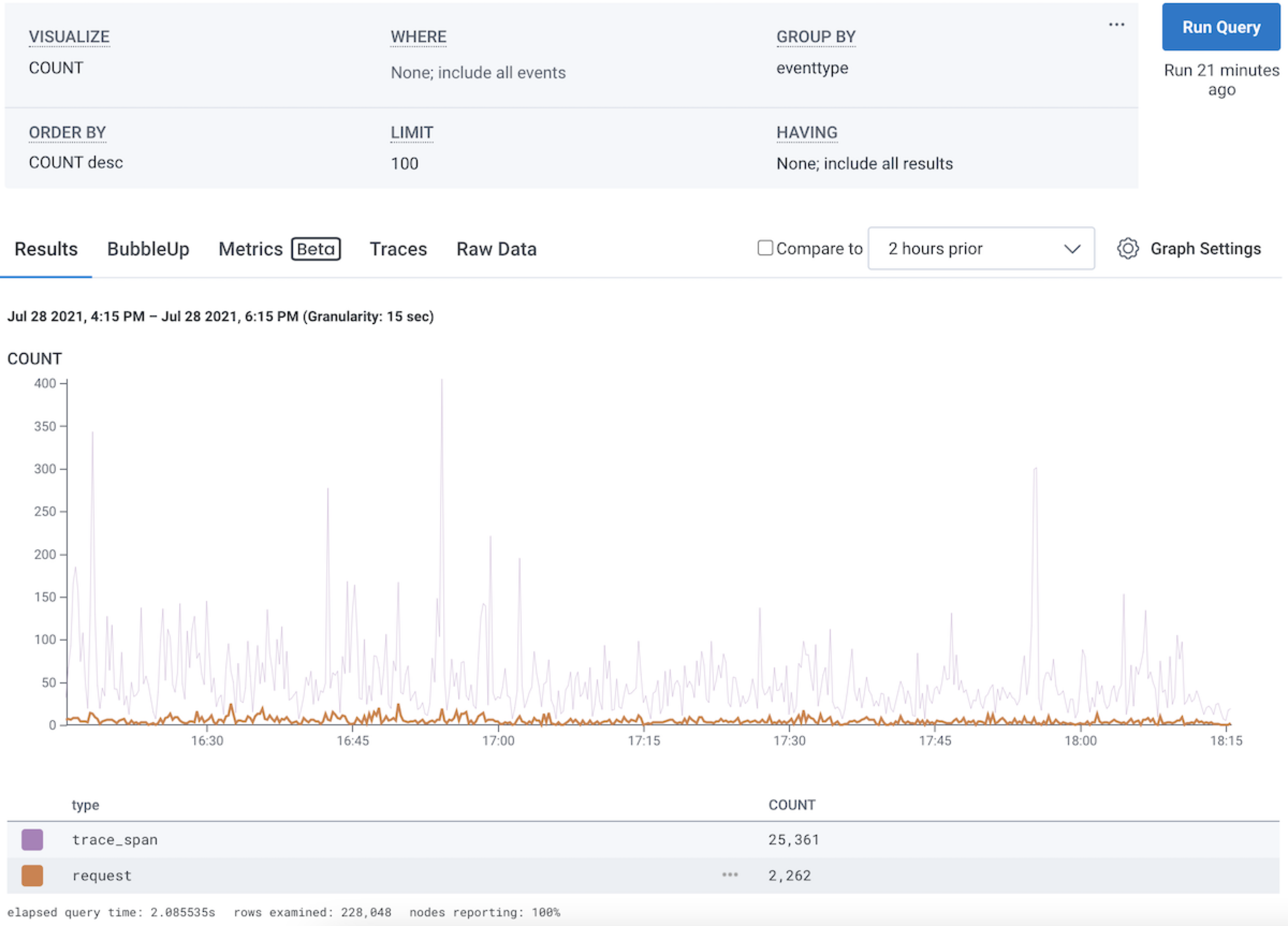
In this figure, the user has a **SELECT** `COUNT`, and **GROUP BY** `eventtype`.
The two curves, in purple and orange, show the two groups.
The popup shows that the user is hovering the `trace_span` eventtype, which has a count of 405 in that 15-second time range.
### Change Datasets
In the upper left corner above the Query Builder, use the **Dataset Switcher** to choose to query a specific Dataset or all Datasets within your Environment.
The latter option may be useful if you need to reference events that span across multiple services.
When you switch datasets, Honeycomb will load the existing query on that dataset, but it will not run it automatically.
You can also set a default scope for new queries per environment in [Environment Settings](/reference/honeycomb-ui/environment/environment-settings/).
### Change and Compare Query Time Ranges
In the bottom right corner below the Query Builder, use the **time picker** to modify the selected time span of the data in your query.
Use a preset time range or a custom time range.
Honeycomb supports running queries across different periods of time, so you can compare results to see how your systems change.
Run a Time Comparison query by selecting a time range under **Compare to previous time period** in the time picker.
Honeycomb then will run a query as defined in the Query Builder and another query for the time comparison range selected.
## Query Reference
### SELECT
Honeycomb supports a wide range of calculations to provide insight into your events.
When a grouping is provided, calculations occur within each group; otherwise, anything calculated is done so over all matching events.
For example, say you have collected the following events from your web server logs:
| Timestamp | uri | status\_code | response\_time\_ms |
| :--------------- | :----- | :----------- | :----------------- |
| 2016-08-01 07:30 | /about | 500 | 126 |
| 2016-08-01 07:45 | /about | 200 | 57 |
| 2016-08-01 07:57 | /docs | 200 | 82 |
| 2016-08-01 08:03 | /docs | 200 | 23 |
Specifying a visualization for a particular attribute (`P95(response_time_ms)`for example) means to apply the aggregation function (in this case, `P95`, or taking the 95th [percentile](https://en.wikipedia.org/wiki/Percentile)) over the values for the attribute (`response_time_ms`) across all input events.
Defining multiple **SELECT** clauses is common and can be useful, especially when comparing their outputs to each other.
For example, it can be useful to see both the `COUNT` and the `P95(duration)` for a set of events to understand whether latency changes follow volume changes.
While most **SELECT** queries return a line graph, the [`HEATMAP`](/investigate/analyze/visualize-events/) visualization allows you see the distribution of data in a rich and interactive way.
Heatmaps also allow you to find outliers in data using [BubbleUp](/investigate/analyze/identify-outliers/).
#### SELECT: Basic Case
Scenario: we want to capture overall statistics for our web server.
Given our four-event dataset [described above](#select), consider a query which contains:
* Visualize the overall `COUNT`
* Visualize the `AVG` of `response_time_ms` values
* Visualize the `P95` of `response_time_ms` values
These calculations would return statistics across the entirety of our dataset:
| COUNT | AVG(response\_time\_ms) | P95(response\_time\_ms) |
| :---- | :---------------------- | :---------------------- |
| 4 | 72 | 119.4 |
#### SELECT: COUNT\_DATAPOINTS
`COUNT_DATAPOINTS` returns the total count of datapoints ingested across all metric fields in a metrics dataset. Use it to understand data volume and track what is driving your usage. The `COUNT_DATAPOINTS` aggregate can only be used with time-series metrics data.
A **datapoint** is a single recorded value for a metric at a point in time, for a unique combination of attributes. Datapoints are the unit by which metrics usage is billed. Every active time series is a unique combination of metric name and attributes, such as `http.server.request.duration` where `k8s.node.name=node-1` which continuously produces datapoints over time. High attribute cardinality means more time series, and therefore more datapoints.
Use `COUNT_DATAPOINTS` to track billing usage over a time range or to spot metric ingestion spikes.
`COUNT_DATAPOINTS` data is only available from February 13, 2026 onward. Queries that include time ranges before this date will only reflect data ingested after that date.
#### SELECT: COUNT\_DATAPOINTS(metric\_field\_name)
`COUNT_DATAPOINTS()` returns the count of datapoints for a specific metric field. Only rows where that column has a value are counted. The `COUNT_DATAPOINTS()` aggregate can only be used with time-series metrics data.
Use this when you want to isolate the datapoint volume of a single metric. For example, comparing ingestion across metrics or identifying which metric is driving a cost increase.
If any metric data has been deleted, `COUNT_DATAPOINTS` will still include those deleted datapoints in its count. `COUNT_DATAPOINTS(metric_field_name)` excludes deleted data.
### SELECT: HISTOGRAM\_COUNT(metric\_field\_name)
`HISTOGRAM_COUNT()` returns the count of observations in a histogram metric field, across the rows and time included in the query.
This aggregate can only be used on time series metrics histogram fields.
#### SELECT Summary Table
The **SELECT** clause returns both a time series graph and a column of values in the result summary table.
Note that in the graph, the values shown are aggregated for each interval at the current granularity.
Conversely, the values shown in the summary table are calculated across the entire time range for that query.
These results can be a little surprising for some calculations.
The `P95(duration_ms)` across the entire time range may not look quite like the `P95` value at any given point of the curve, because there may be spikes and bumps in the underlying data that are hidden in the time intervals.
The summary table for a `HEATMAP` shows a histogram of values of that field across the full time range.
#### SELECT Operations
Most **SELECT** operations take a single argument, with the exception of `COUNT` and `COUNT_DATAPOINTS`, that optionally take an argument, and `CONCURRENCY`, which takes no arguments.
Events that do not have a relevant attribute are ignored, and will not be counted in aggregations.
In the chart below, `` refers to any field name while the `` argument refers to a float or integer field.
| Aggregate | Meaning |
| ------------------------------------------------ | -------------------------------------------------------------------------------------------------------------------------------------------------------------------------------------------------------- |
| `COUNT` | The number of events |
| `COUNT()` | The number of events with a non-null value for a field |
| `COUNT_DISTINCT()` | The count of different distinct values in a field. `COUNT_DISTINCT` is estimated using the HyperLogLog algorithm. |
| `COUNT_DATAPOINTS` | The total count of datapoints ingested across all metric fields in a metrics dataset. |
| `COUNT_DATAPOINTS()` | The count of datapoints for a specified metric field in a metrics dataset. Only rows where the specified field has a value are counted. |
| `HISTOGRAM_COUNT()` | The count of observations recorded in a specified histogram field. Requires a histogram field in a time series metrics dataset as the parameter. |
| `SUM()` | The sum of the field value |
| `AVG()` | The average value of the field |
| `MAX()` | The maximum value of the field |
| `MIN()` | The minimum value of the field |
| `P001()` | The .1-th percentile of the field. `P001` is estimated using the t-digest algorithm. |
| `P01()` | The 1st percentile of the field. `P01` is estimated using the t-digest algorithm. |
| `P05()` | The 5th percentile of the field. `P05` is estimated using the t-digest algorithm. |
| `P10()` | The 10th percentile of the field. `P10` is estimated using the t-digest algorithm. |
| `P20()` | The 20th percentile of the field. `P20` is estimated using the t-digest algorithm. |
| `P25()` | The 25th percentile of the field. `P25` is estimated using the t-digest algorithm. |
| `P50()` | The 50th percentile of the field. `P50` is estimated using the t-digest algorithm. |
| `P75()` | The 75th percentile of the field. `P75` is estimated using the t-digest algorithm. |
| `P80()` | The 80th percentile of the field. `P80` is estimated using the t-digest algorithm. |
| `P90()` | The 90th percentile of the field. `P90` is estimated using the t-digest algorithm. |
| `P95()` | The 95th percentile of the field. `P95` is estimated using the t-digest algorithm. |
| `P99()` | The 99th percentile of the field. `P99` is estimated using the t-digest algorithm. |
| `P999()` | The 99.9th percentile of the field. `P999` is estimated using the t-digest algorithm. |
| `HEATMAP()` | A heatmap of the distribution of that field |
| `CONCURRENCY` | The concurrency of the current query, for tracing-enabled datasets only. This is a complex operation; please see the [detailed explanatory page](/investigate/query/build/visualize-concurrency/) on it. |
| `RATE_AVG()` | The difference between subsequent field values after applying the `RATE_AVG` operator. [Learn more about the RATE operators](/investigate/query/build/visualize-rate/). |
| `RATE_SUM()` | The difference between subsequent field values after applying the `RATE_SUM` operator. [Learn more about the RATE operators](/investigate/query/build/visualize-rate/). |
| `RATE_MAX()` | The difference between subsequent field values after applying the `RATE_MAX` operator. [Learn more about the RATE operators](/investigate/query/build/visualize-rate/). |
### WHERE
The **WHERE** clause allows you to constrain events by some attribute besides time. For example, you may want to ignore an outlier case or isolate events triggered by a particular actor or circumstance.
For example, say you have collected the following events from your web server logs:
| Timestamp | uri | status\_code |
| :--------------- | :----- | :----------- |
| 2016-08-01 08:15 | /about | 500 |
| 2016-08-01 08:22 | /about | 200 |
| 2016-08-01 08:27 | /docs | 403 |
You can define any number of arbitrary constraints based on event values.
**WHERE** clauses work in concert with the specified time range to define the events that are ultimately considered by any **GROUP BY** or **SELECT** clauses.
The **WHERE** clause does not require string delimiters or escape characters. For example, to match a URI of `/docs`, you can enter `uri = /docs`.
#### WHERE: Basic Case
Scenario: we want to understand the frequency of unsuccessful web requests.
Given our three-event dataset [described above](#where), consider a query which contains:
* **SELECT** the overall `COUNT`
* **WHERE** `status_code != 200`
The **WHERE** clause removes the successful event (our `/about` web request returning a `200`) from consideration, and only counts the first and third events towards our **SELECT** clause:
| COUNT |
| :---- |
| 2 |
#### WHERE: Multiple Clauses
Scenario: we want to refine our constraints further, to span multiple attributes for each event.
Combining **WHERE** clauses returns events that satisfy either the **intersection** of all specified **WHERE** clauses, or the **union**.
Given our three-event dataset [described above](#where), consider a query which contains:
* Where `uri = "/about"`
* AND `status_code != 200`
As all three events are considered by the **WHERE** clauses, only the first one satisfies both:
| Timestamp | uri | status\_code |
| :--------------- | :----- | :----------- |
| 2016-08-01 08:55 | /about | 500 |
Honeycomb also allows you to look at the **union** of clauses by setting to an `OR`.
* **WHERE** `status_code = 500`
* OR `status_code = 403`
| Timestamp | uri | status\_code |
| :--------------- | :----- | :----------- |
| 2016-08-01 08:55 | /about | 500 |
| 2016-08-01 08:27 | /docs | 403 |
#### WHERE: Relational Fields
You can use relational fields in your **WHERE** clause to narrow your query to find traces that contain fields and values within a specific span type.
To learn more and explore some examples, visit [Relational Fields](#relational-fields-1) in this reference.
#### WHERE Operations
`WHERE` operations may take one or more attributes.
Events are only counted if they have a relevant attribute, except in the case of the `does-not-exist` operation.
| Operation | Opposite | Arguments | Meaning |
| :------------ | :-------------------- | :-------- | :------------------------------------------------------------------------------ |
| `=` | `!=` | 1 | Exact numerical or string match |
| `starts-with` | `does-not-start-with` | 1 | String start match |
| `ends-with` | `does-not-end-with` | 1 | String end match |
| `exists` | `does-not-exist` | 0 | Checks for non-null values |
| `>`, `>=` | `<`, `<=` | 1 | numerical comparison |
| `contains` | `does-not-contain` | 1 | string inclusion: checks whether the attribute matches a substring of the value |
| `in` | `not-in` | 1+ | list inclusion: checks whether the attribute matches any item in the list |
The syntax for the `in` operator does not use parentheses.
For example, `request_method in GET,POST`
### GROUP BY
Being able to separate a series of events into groups by attribute is a powerful way to compare segments of your dataset against each other.
For example, say you have collected the following events from your web server logs:
| Timestamp | uri | status\_code |
| :--------------- | :----- | :----------- |
| 2016-08-01 07:30 | /about | 500 |
| 2016-08-01 07:45 | /about | 200 |
| 2016-08-01 07:57 | /docs | 200 |
You might want to analyze your web traffic in groups based on the `uri` ("/about" vs "/docs") or the `status_code` (`500` versus `200`).
Choosing to group by `uri` would return two result rows: one representing events in which `uri="/about"` and another representing events in which `uri="/docs"`.
Each of these grouped results rows will be represented by a single line on a graph.
When using GROUP BY for more than one attribute, Honeycomb will consider each unique combination of values as a single group.
Here, choosing to group by both `uri` and `status_code` will return three groups: `/about`+`500`, `/about`+`200`, and `/docs`+`200`.
Grouping, paired with calculation, can often reveal interesting patterns in your underlying events—grouping by `uri`, for example, and calculating response time stats will show you the slowest (or fastest) `uri`s.
Honeycomb supports grouping your data based on any attribute in an event, though you will likely receive the clearest results by choosing an attribute with an uneven distribution within your data.
The **GROUP BY** dropdown list also has a shortcut to [create a calculated field](/configure/environments/calculated-fields/).
#### Grouping and Selecting: Better Together
Scenario: we want to examine performance of our web server by endpoint.
Given our four-event dataset [described above](#select), consider a query which contains:
* Group by `uri`
* Select the overall `COUNT`
* Select the `AVG` of `response_time_ms` values
Pairing a Grouping clause with a Select clause results in events being grouped by `uri`; Honeycomb draws one line for each group, and calculates statistics within each group:
| uri | COUNT | AVG(response\_time\_ms) |
| :----- | :---- | :---------------------- |
| /about | 2 | 91.5 |
| /docs | 2 | 52.5 |
This technique is particularly powerful when paired with an Order By and a Limit to return "Top K"-style results.
In this figure, the user has a **SELECT** `COUNT`, and **GROUP BY** `eventtype`.
The two curves, in purple and orange, show the two groups.
The popup shows that the user is hovering the `trace_span` eventtype, which has a count of 405 in that 15-second time range.
 When you move your cursor over the results table at the bottom of the page, each row is highlighted in turn.
In the image below, the user has highlighted `request` and sees the orange line highlighted, and the purple line dimmed.
When you move your cursor over the results table at the bottom of the page, each row is highlighted in turn.
In the image below, the user has highlighted `request` and sees the orange line highlighted, and the purple line dimmed.
 Rollover for heatmaps is slightly different, as described on the [Heatmaps](/investigate/analyze/visualize-events/) page.
**50-Series Visualization Limit**: Honeycomb visualizes only the top 50 groups by the selected aggregation (e.g., MAX, MIN, AVG) in graphs, regardless of the **LIMIT** clause value. The **LIMIT** clause controls how many rows appear in the results table, but we will only ever show up to the top 50 groups as series in the visualization. When you change the time range, the visualized groups will change based on the query's sort clause and the total value of each aggregation within the query's time range, which can cause series to appear or disappear when zooming in or out.
**Time Bucket Edge Effects**: The first and last data points in a graph may represent shorter time intervals when query boundaries don't align with the selected granularity. For example, with 2-minute granularity and a query ending at 08:32:44, the bucket for 08:32:00 will only contain 44 seconds of data, which can make it look like data is missing or dropping unexpectedly at the edges of graphs.
#### GROUP BY: Relational Fields
You can use relational fields in your **GROUP BY** clause to separate a series of events into groups.
To learn more and explore some examples, visit [Relational Fields](#relational-fields-1) in this reference.
### ORDER BY
**ORDER BY** clauses define how rows will be sorted in the results table.
For example, say you have collected the following events from your web server logs:
| Timestamp | uri | status\_code | response\_time\_ms |
| :--------------- | :----- | :----------- | :----------------- |
| 2016-08-01 09:17 | /about | 200 | 57 |
| 2016-08-01 09:18 | /about | 500 | 234 |
| 2016-08-01 09:20 | /404 | 200 | 12 |
| 2016-08-01 09:25 | /docs | 200 | 82 |
You can define any number of **ORDER BY** clauses in a query and they will be respected in the order they are specified.
The **ORDER BY** clauses available to you for a particular query are influenced by whether any **GROUP BY** or **SELECT** clauses are also specified.
If none are, you may order by any of the attributes contained in the dataset.
However, once a **GROUP BY** or **SELECT** clause exists, you may only order by the values generated by those clauses.
#### ORDER BY: Basic Case
Scenario: we just want to get a sense of the slowest endpoints in our web server.
Given our four-event dataset [described above](#order-by), consider a query which contains:
* Order by `response_time_ms` in descending (`DESC`) order
* Limit to 1 result
Remember that when no Select clauses are defined, we simply return raw events as the result rows:
| Timestamp | uri | status\_code | response\_time\_ms |
| :--------------- | :----- | :----------- | :----------------- |
| 2016-08-01 09:18 | /about | 500 | 234 |
#### ORDER BY as Paired with SELECT and GROUP BY Clauses
Scenario: we want to capture statistics for our web server and know what we are looking for (long `response_time_ms`s).
Given our four-event dataset [described above](#order-by), consider a query which contains:
* **SELECT** `P95(response_time_ms)`, or the p95 of `response_time_ms` values
* **GROUP BY** `uri`
* **ORDER BY** `P95(response_time_ms)` in descending (`DESC`) order
* **LIMIT** to the first `2` results
Our **GROUP BY** and **SELECT** queries influence **what** will be returned as result rows (`uri` and the `P95(response_time_ms)` for events within each distinct `uri` group), while the **ORDER BY** determines the sort order of those results (longest `P95(response_time_ms)` first) and the **LIMIT** throws away any results beyond the top `2`:
| uri | P95(response\_time\_ms) |
| :----- | :---------------------- |
| /about | 225.15 |
| /docs | 82 |
As you can see, any results referencing the event with `uri="/404"` was excluded from our result set as a result of its relatively low `response_time_ms`.
This sort of Top K query is particularly valuable when working with high-cardinality data sets, where a **GROUP BY** clause might split your dataset into a very large number of groups.
### LIMIT
The **LIMIT** clause provides a maximum number of result rows to return.
By default, queries return 100 result rows.
The **LIMIT** clause allows you to specify up to 1000 rows.
### HAVING
The **HAVING** clause allows you to filter on the results table.
This operation is distinct from the **WHERE** clause, which filters the underlying events.
A **HAVING** filter can help further refine your query results when grouping on a high-cardinality attribute, which can result in many different rows in the result table.
It can also work in tandem with an **ORDER BY** clause.
**ORDER BY** allows you to order the results, and **HAVING** filters them.
Like **ORDER BY**, **HAVING** selects its series from the results table.
For example, consider a query on **SELECT** `COUNT, P95(duration_ms)` and **GROUP BY** `endpoint`.
This query would show how many times each endpoint ran, and how often it did so.
The results table from this query might look something like this:
| endpoint | COUNT | P95(duration\_ms) |
| :---------------- | :---- | :---------------- |
| /add-to-cart | 521 | 45 |
| /remove-from-cart | 1021 | 54 |
| /unused-endpoint | 2 | 1500 |
| /empty-page | 10 | 1700 |
You might want to ignore the rarest entries when they are least likely to be useful.
One way to do that is to add a **HAVING** clause:
The clause **HAVING** `COUNT > 100` will filter to only results with more than 100 hits on them.
You can then **ORDER BY** `P95( duration_ms )` to sort the results to find the slowest endpoints.
**HAVING** works by filtering specifically on aggregations across all results in the selected time range.
It currently does not filter time periods that match the criteria.
Take a look at the following example.
Each event has counts ranging from 0 - 9 across the time range.
Rollover for heatmaps is slightly different, as described on the [Heatmaps](/investigate/analyze/visualize-events/) page.
**50-Series Visualization Limit**: Honeycomb visualizes only the top 50 groups by the selected aggregation (e.g., MAX, MIN, AVG) in graphs, regardless of the **LIMIT** clause value. The **LIMIT** clause controls how many rows appear in the results table, but we will only ever show up to the top 50 groups as series in the visualization. When you change the time range, the visualized groups will change based on the query's sort clause and the total value of each aggregation within the query's time range, which can cause series to appear or disappear when zooming in or out.
**Time Bucket Edge Effects**: The first and last data points in a graph may represent shorter time intervals when query boundaries don't align with the selected granularity. For example, with 2-minute granularity and a query ending at 08:32:44, the bucket for 08:32:00 will only contain 44 seconds of data, which can make it look like data is missing or dropping unexpectedly at the edges of graphs.
#### GROUP BY: Relational Fields
You can use relational fields in your **GROUP BY** clause to separate a series of events into groups.
To learn more and explore some examples, visit [Relational Fields](#relational-fields-1) in this reference.
### ORDER BY
**ORDER BY** clauses define how rows will be sorted in the results table.
For example, say you have collected the following events from your web server logs:
| Timestamp | uri | status\_code | response\_time\_ms |
| :--------------- | :----- | :----------- | :----------------- |
| 2016-08-01 09:17 | /about | 200 | 57 |
| 2016-08-01 09:18 | /about | 500 | 234 |
| 2016-08-01 09:20 | /404 | 200 | 12 |
| 2016-08-01 09:25 | /docs | 200 | 82 |
You can define any number of **ORDER BY** clauses in a query and they will be respected in the order they are specified.
The **ORDER BY** clauses available to you for a particular query are influenced by whether any **GROUP BY** or **SELECT** clauses are also specified.
If none are, you may order by any of the attributes contained in the dataset.
However, once a **GROUP BY** or **SELECT** clause exists, you may only order by the values generated by those clauses.
#### ORDER BY: Basic Case
Scenario: we just want to get a sense of the slowest endpoints in our web server.
Given our four-event dataset [described above](#order-by), consider a query which contains:
* Order by `response_time_ms` in descending (`DESC`) order
* Limit to 1 result
Remember that when no Select clauses are defined, we simply return raw events as the result rows:
| Timestamp | uri | status\_code | response\_time\_ms |
| :--------------- | :----- | :----------- | :----------------- |
| 2016-08-01 09:18 | /about | 500 | 234 |
#### ORDER BY as Paired with SELECT and GROUP BY Clauses
Scenario: we want to capture statistics for our web server and know what we are looking for (long `response_time_ms`s).
Given our four-event dataset [described above](#order-by), consider a query which contains:
* **SELECT** `P95(response_time_ms)`, or the p95 of `response_time_ms` values
* **GROUP BY** `uri`
* **ORDER BY** `P95(response_time_ms)` in descending (`DESC`) order
* **LIMIT** to the first `2` results
Our **GROUP BY** and **SELECT** queries influence **what** will be returned as result rows (`uri` and the `P95(response_time_ms)` for events within each distinct `uri` group), while the **ORDER BY** determines the sort order of those results (longest `P95(response_time_ms)` first) and the **LIMIT** throws away any results beyond the top `2`:
| uri | P95(response\_time\_ms) |
| :----- | :---------------------- |
| /about | 225.15 |
| /docs | 82 |
As you can see, any results referencing the event with `uri="/404"` was excluded from our result set as a result of its relatively low `response_time_ms`.
This sort of Top K query is particularly valuable when working with high-cardinality data sets, where a **GROUP BY** clause might split your dataset into a very large number of groups.
### LIMIT
The **LIMIT** clause provides a maximum number of result rows to return.
By default, queries return 100 result rows.
The **LIMIT** clause allows you to specify up to 1000 rows.
### HAVING
The **HAVING** clause allows you to filter on the results table.
This operation is distinct from the **WHERE** clause, which filters the underlying events.
A **HAVING** filter can help further refine your query results when grouping on a high-cardinality attribute, which can result in many different rows in the result table.
It can also work in tandem with an **ORDER BY** clause.
**ORDER BY** allows you to order the results, and **HAVING** filters them.
Like **ORDER BY**, **HAVING** selects its series from the results table.
For example, consider a query on **SELECT** `COUNT, P95(duration_ms)` and **GROUP BY** `endpoint`.
This query would show how many times each endpoint ran, and how often it did so.
The results table from this query might look something like this:
| endpoint | COUNT | P95(duration\_ms) |
| :---------------- | :---- | :---------------- |
| /add-to-cart | 521 | 45 |
| /remove-from-cart | 1021 | 54 |
| /unused-endpoint | 2 | 1500 |
| /empty-page | 10 | 1700 |
You might want to ignore the rarest entries when they are least likely to be useful.
One way to do that is to add a **HAVING** clause:
The clause **HAVING** `COUNT > 100` will filter to only results with more than 100 hits on them.
You can then **ORDER BY** `P95( duration_ms )` to sort the results to find the slowest endpoints.
**HAVING** works by filtering specifically on aggregations across all results in the selected time range.
It currently does not filter time periods that match the criteria.
Take a look at the following example.
Each event has counts ranging from 0 - 9 across the time range.
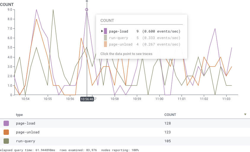 You may want to filter specifically on counts greater than 5 in the example and add the clause **HAVING** `COUNT > 5`.
This will still return all results in the image, since **HAVING** filters based off the total in the result table where all values are shown to have counts > 5.
#### HAVING Clause Options
The **HAVING** clause always refers to one of the **SELECT** clauses.
It then takes one or more numeric arguments.
| Operator | Opposite | Arguments | Meaning |
| -------- | -------- | --------- | ------------------- |
| = | != | 1 | numerical equality |
| >, >= | \<, \<= | 1 | comparison |
| in | not-in | 1+ | existence in a list |
The `in` operator compares where a value is one of a set: `COUNT in 10, 20, 30` checks whether the COUNT is precisely one of those values.
The syntax for the `in` operator does not use parentheses.
### Relational Fields
You can use relational fields to narrow your query to find traces that contain fields and values within a specific span type.
Span types are identified by prefixes that follow your trace structure.
You can use relational fields in **WHERE** or **GROUP BY** clauses in the Honeycomb UI.
If you use relational fields, your conditions will be joined using **AND** operators by default.
To make your queries run faster, add filters to narrow possible matches.
Filtering on joined events is particularly helpful.
For example, if you include a filter like `any.name = foo`, also include a filter like `any.service_name = bar`.
Adding the additional filter keeps us from searching your entire environment, which lets us speed things up!
To learn about more best practices, visit [Best Practices for Querying using Relational Fields](/get-started/best-practices/relational-fields/).
#### Prefix: root
The `root.` prefix matches to the root span within a trace.
When you use it, additional filters in your query will match only for spans in traces that match the conditions on the root span.
You can also query with `root.` on its own.
If you are looking for spans somewhere in a trace that you know starts with certain fields, use `root.`.
So you might use a query that contains:
* **SELECT** `COUNT`
* **WHERE** `name = HGET` AND `root.name = /cart` AND `root.duration_ms > 1000`
You may want to filter specifically on counts greater than 5 in the example and add the clause **HAVING** `COUNT > 5`.
This will still return all results in the image, since **HAVING** filters based off the total in the result table where all values are shown to have counts > 5.
#### HAVING Clause Options
The **HAVING** clause always refers to one of the **SELECT** clauses.
It then takes one or more numeric arguments.
| Operator | Opposite | Arguments | Meaning |
| -------- | -------- | --------- | ------------------- |
| = | != | 1 | numerical equality |
| >, >= | \<, \<= | 1 | comparison |
| in | not-in | 1+ | existence in a list |
The `in` operator compares where a value is one of a set: `COUNT in 10, 20, 30` checks whether the COUNT is precisely one of those values.
The syntax for the `in` operator does not use parentheses.
### Relational Fields
You can use relational fields to narrow your query to find traces that contain fields and values within a specific span type.
Span types are identified by prefixes that follow your trace structure.
You can use relational fields in **WHERE** or **GROUP BY** clauses in the Honeycomb UI.
If you use relational fields, your conditions will be joined using **AND** operators by default.
To make your queries run faster, add filters to narrow possible matches.
Filtering on joined events is particularly helpful.
For example, if you include a filter like `any.name = foo`, also include a filter like `any.service_name = bar`.
Adding the additional filter keeps us from searching your entire environment, which lets us speed things up!
To learn about more best practices, visit [Best Practices for Querying using Relational Fields](/get-started/best-practices/relational-fields/).
#### Prefix: root
The `root.` prefix matches to the root span within a trace.
When you use it, additional filters in your query will match only for spans in traces that match the conditions on the root span.
You can also query with `root.` on its own.
If you are looking for spans somewhere in a trace that you know starts with certain fields, use `root.`.
So you might use a query that contains:
* **SELECT** `COUNT`
* **WHERE** `name = HGET` AND `root.name = /cart` AND `root.duration_ms > 1000`
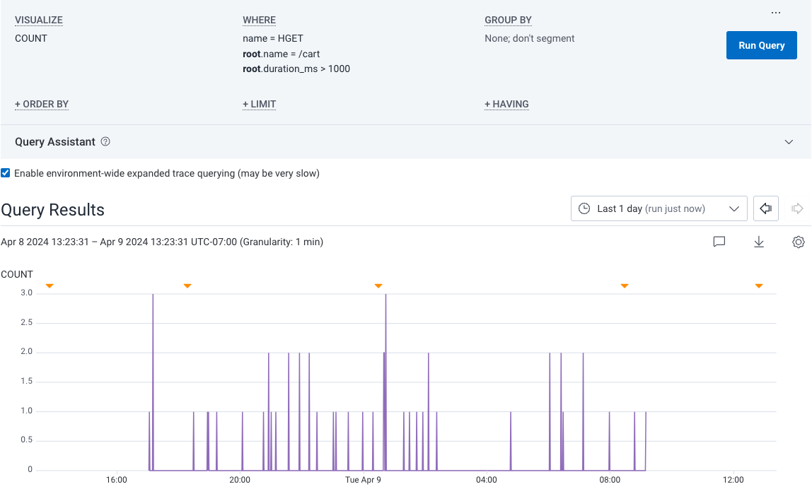 And you might see the following trace summary when you select a span from the query results:
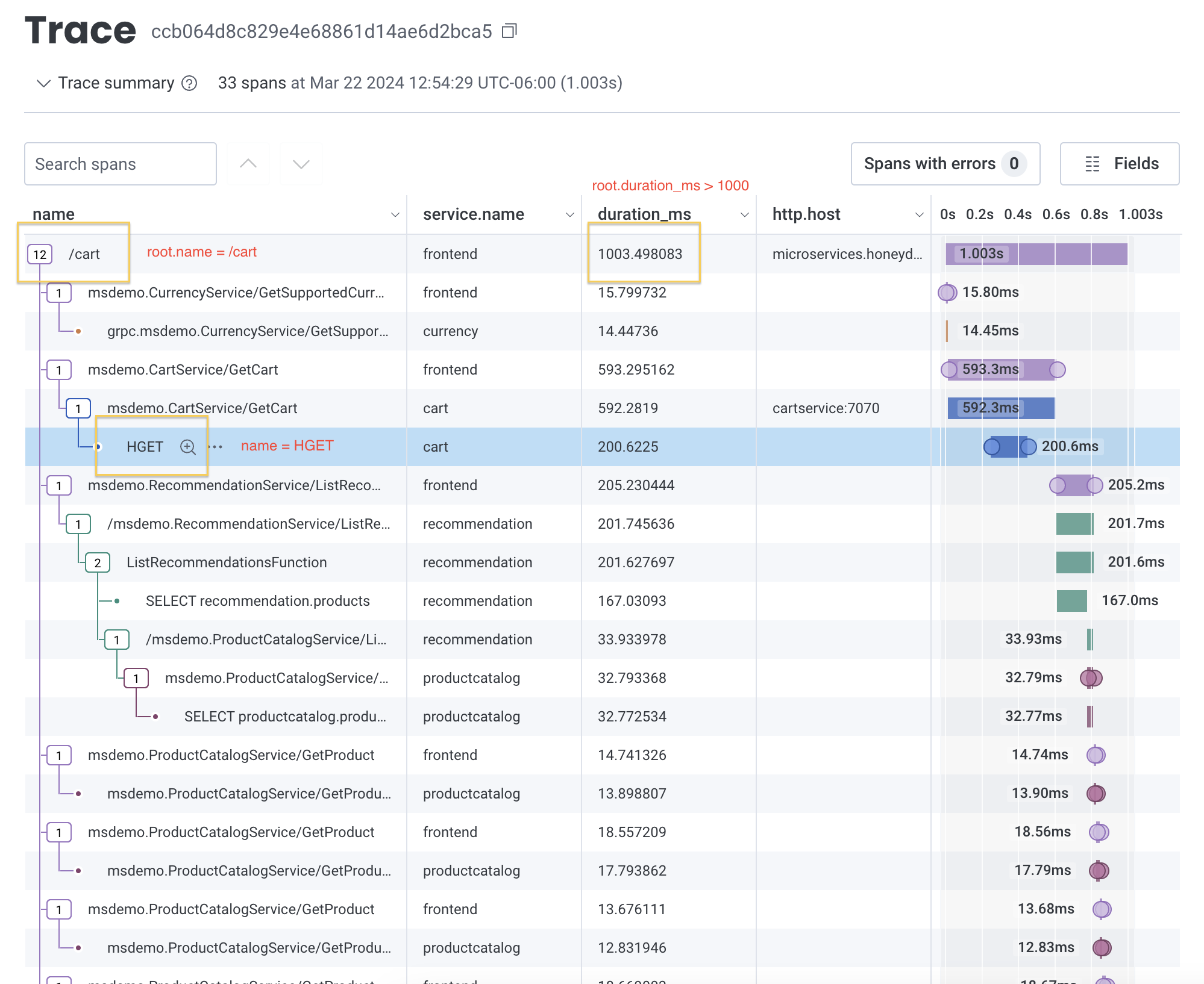 To explore more examples related to using relational fields with the `root.` prefix, visit [Examples: Query for Traces](/investigate/query/examples-traces/#root-prefix).
#### Prefix: parent
The `parent.` prefix matches to a direct parent span within a trace.
When you use it, additional filters in your query will search through fields only in the specified `parent.` span's immediate child spans.
For example, if you know a service is being called at a lower level inside a trace, and you want to find one of its direct child spans, use `parent.`.
You can also use `parent.` with no additional filters to count the child spans of a parent span.
When you do so, Honeycomb will match to one parent span per trace.
So you might use a query that contains:
* **SELECT** `COUNT`
* **WHERE** `status_message exists` AND `parent.service.name = frontend`
* **GROUP BY** `status_message` `service.name` `name`
To explore more examples related to using relational fields with the `root.` prefix, visit [Examples: Query for Traces](/investigate/query/examples-traces/#root-prefix).
#### Prefix: parent
The `parent.` prefix matches to a direct parent span within a trace.
When you use it, additional filters in your query will search through fields only in the specified `parent.` span's immediate child spans.
For example, if you know a service is being called at a lower level inside a trace, and you want to find one of its direct child spans, use `parent.`.
You can also use `parent.` with no additional filters to count the child spans of a parent span.
When you do so, Honeycomb will match to one parent span per trace.
So you might use a query that contains:
* **SELECT** `COUNT`
* **WHERE** `status_message exists` AND `parent.service.name = frontend`
* **GROUP BY** `status_message` `service.name` `name`
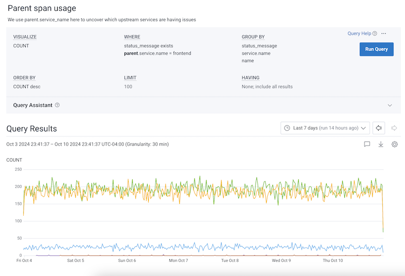 And you might see the following trace summary when you select a span from the query results:
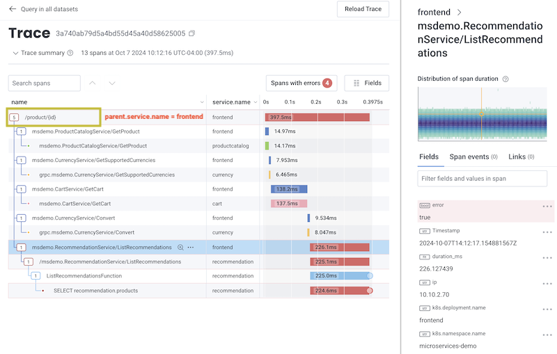 To explore more examples related to using relational fields with the `parent.` prefix, visit [Examples: Query for Traces](/investigate/query/examples-traces/#parent-prefix).
#### Prefix: child
The `child.` prefix matches to a direct child span within a trace.
When you use it, additional filters in your query will search through fields only in the specified `child.` span.
For example, if you know a service is being called on a specific lower-level span inside a trace, and you want to search only that span, use `child.`.
* If you use multiple `child.` relational fields in the same clause, Honeycomb will apply them all to the same span.
* `child.` returns results in random order.
So you might use a query that contains:
* **SELECT** `COUNT`
* **WHERE** `name = /cart`
* **GROUP BY** `child.name`
To explore more examples related to using relational fields with the `parent.` prefix, visit [Examples: Query for Traces](/investigate/query/examples-traces/#parent-prefix).
#### Prefix: child
The `child.` prefix matches to a direct child span within a trace.
When you use it, additional filters in your query will search through fields only in the specified `child.` span.
For example, if you know a service is being called on a specific lower-level span inside a trace, and you want to search only that span, use `child.`.
* If you use multiple `child.` relational fields in the same clause, Honeycomb will apply them all to the same span.
* `child.` returns results in random order.
So you might use a query that contains:
* **SELECT** `COUNT`
* **WHERE** `name = /cart`
* **GROUP BY** `child.name`
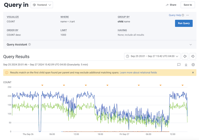 And you might see the following trace summary when you select a span from the query results:
 To explore more examples related to using relational fields with the `child.` prefix, visit [Examples: Query for Traces](/investigate/query/examples-traces/#child-prefix).
#### Prefix: anyX
The `anyX.` prefixes (`any.`, `any2.`, `any3.`) match to a single span anywhere within a trace.
Use `anyX.` prefixes together to query for a trace that contains up to three spans, each with their own filters.
When you use an `anyX.` prefix, additional filters in your query will apply only to the same matched span.
If you are using an `anyX.` prefix in your GROUP BY clause, you must also use the same `anyX.` prefix in your **WHERE** clause.
Doing so will ensure your joins are accurate.
* If you use multiple `anyX.` relational fields in the same clause, Honeycomb will apply them all to the same span.
* `anyX.` returns results in random order.
So you might use a query that contains:
* **SELECT** `COUNT`
* **WHERE** `name = getDiscounts` AND `any.http.host = cartservice:7070` AND `any.duration_ms > 100`
To explore more examples related to using relational fields with the `child.` prefix, visit [Examples: Query for Traces](/investigate/query/examples-traces/#child-prefix).
#### Prefix: anyX
The `anyX.` prefixes (`any.`, `any2.`, `any3.`) match to a single span anywhere within a trace.
Use `anyX.` prefixes together to query for a trace that contains up to three spans, each with their own filters.
When you use an `anyX.` prefix, additional filters in your query will apply only to the same matched span.
If you are using an `anyX.` prefix in your GROUP BY clause, you must also use the same `anyX.` prefix in your **WHERE** clause.
Doing so will ensure your joins are accurate.
* If you use multiple `anyX.` relational fields in the same clause, Honeycomb will apply them all to the same span.
* `anyX.` returns results in random order.
So you might use a query that contains:
* **SELECT** `COUNT`
* **WHERE** `name = getDiscounts` AND `any.http.host = cartservice:7070` AND `any.duration_ms > 100`
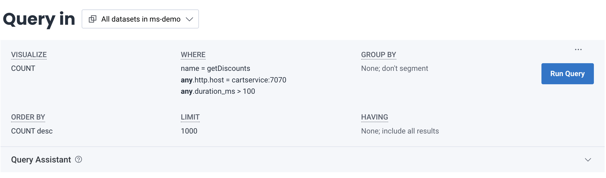 And you might see the following trace summary when you select a span from the query results:
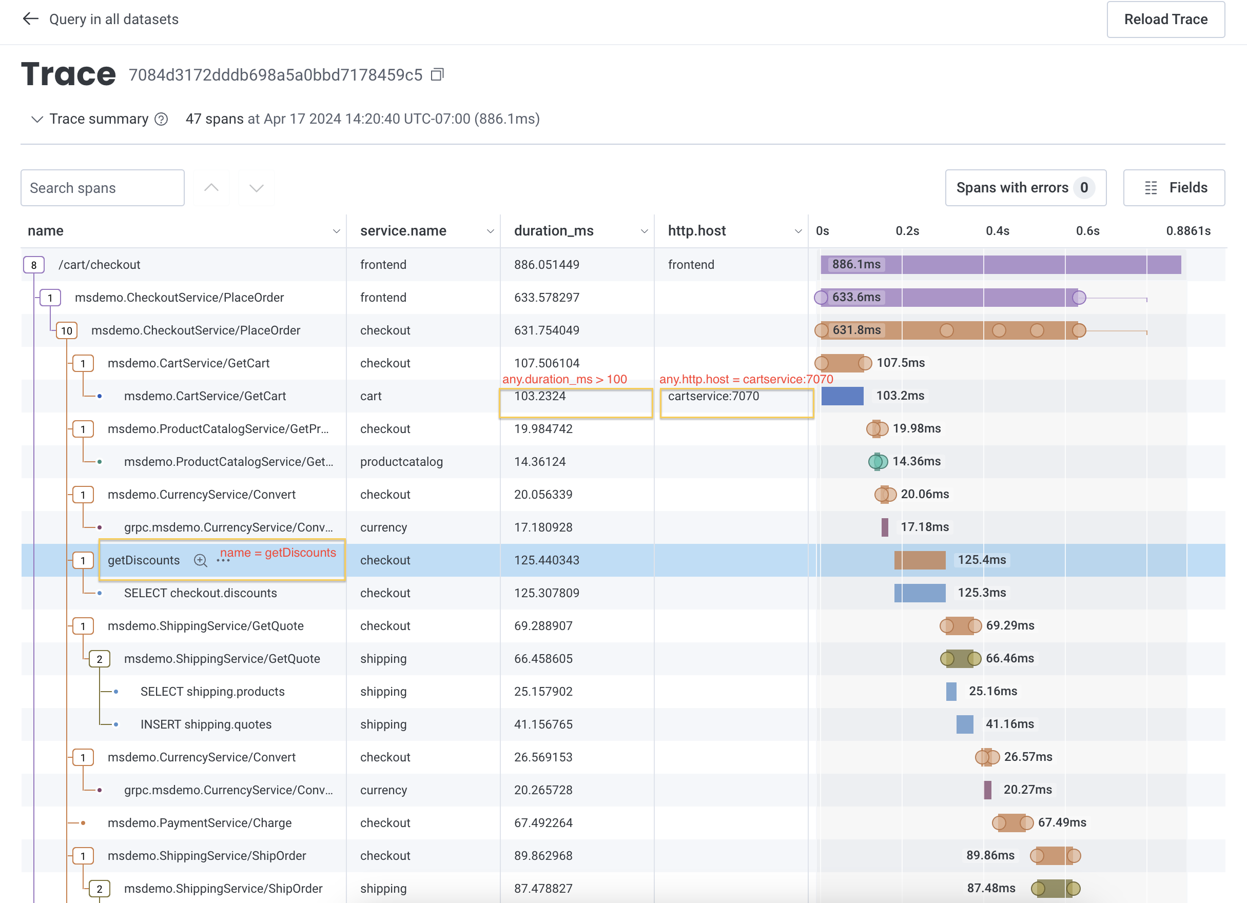 To explore more examples related to using relational fields with the `anyX.` prefix, visit [Examples: Query for Traces](/investigate/query/examples-traces/#anyx-prefix).
#### Prefix: none
The `none.` prefix matches to a single span and excludes any traces that contain the matched span.
When you use it, additional filters in your query will search through only fields not in the matched `none.` span.
* If you use multiple `none.` relational fields in the WHERE clause, Honeycomb will apply them all to the same span.
* `none.` is not available in the GROUP BY clause.
So you might use a query that contains:
* **SELECT** `COUNT`
* **WHERE** `none.trace.parent_id does-not-exist`
* **GROUP BY** `trace.trace_id`
To explore more examples related to using relational fields with the `anyX.` prefix, visit [Examples: Query for Traces](/investigate/query/examples-traces/#anyx-prefix).
#### Prefix: none
The `none.` prefix matches to a single span and excludes any traces that contain the matched span.
When you use it, additional filters in your query will search through only fields not in the matched `none.` span.
* If you use multiple `none.` relational fields in the WHERE clause, Honeycomb will apply them all to the same span.
* `none.` is not available in the GROUP BY clause.
So you might use a query that contains:
* **SELECT** `COUNT`
* **WHERE** `none.trace.parent_id does-not-exist`
* **GROUP BY** `trace.trace_id`
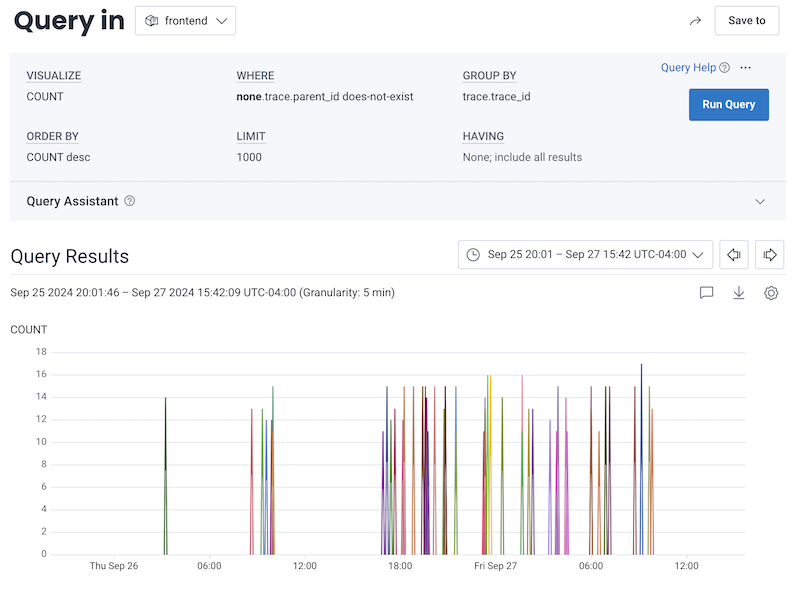 And you might see the following trace summary when you select a span from the query results:
 To explore more examples related to using relational fields with the `none.` prefix, visit [Examples: Query for Traces](/investigate/query/examples-traces/#none-prefix).
#### Example: Using Relational Fields Prefixes Together
You can use all of the relational fields prefixes together to perform a more complex query.
So you might use a query that contains:
* **SELECT** `COUNT`
* **WHERE** `error exists` AND `root.name = /cart/checkout` AND `parent.duration_ms > 200` AND `any.name = getDiscounts`
* **GROUP BY** `any.k8s.pod.name`
To explore more examples related to using relational fields with the `none.` prefix, visit [Examples: Query for Traces](/investigate/query/examples-traces/#none-prefix).
#### Example: Using Relational Fields Prefixes Together
You can use all of the relational fields prefixes together to perform a more complex query.
So you might use a query that contains:
* **SELECT** `COUNT`
* **WHERE** `error exists` AND `root.name = /cart/checkout` AND `parent.duration_ms > 200` AND `any.name = getDiscounts`
* **GROUP BY** `any.k8s.pod.name`
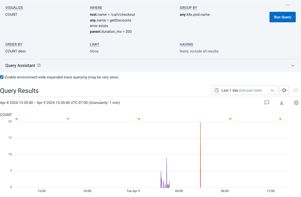 And you might see the following trace summary when you select a span from the query results:
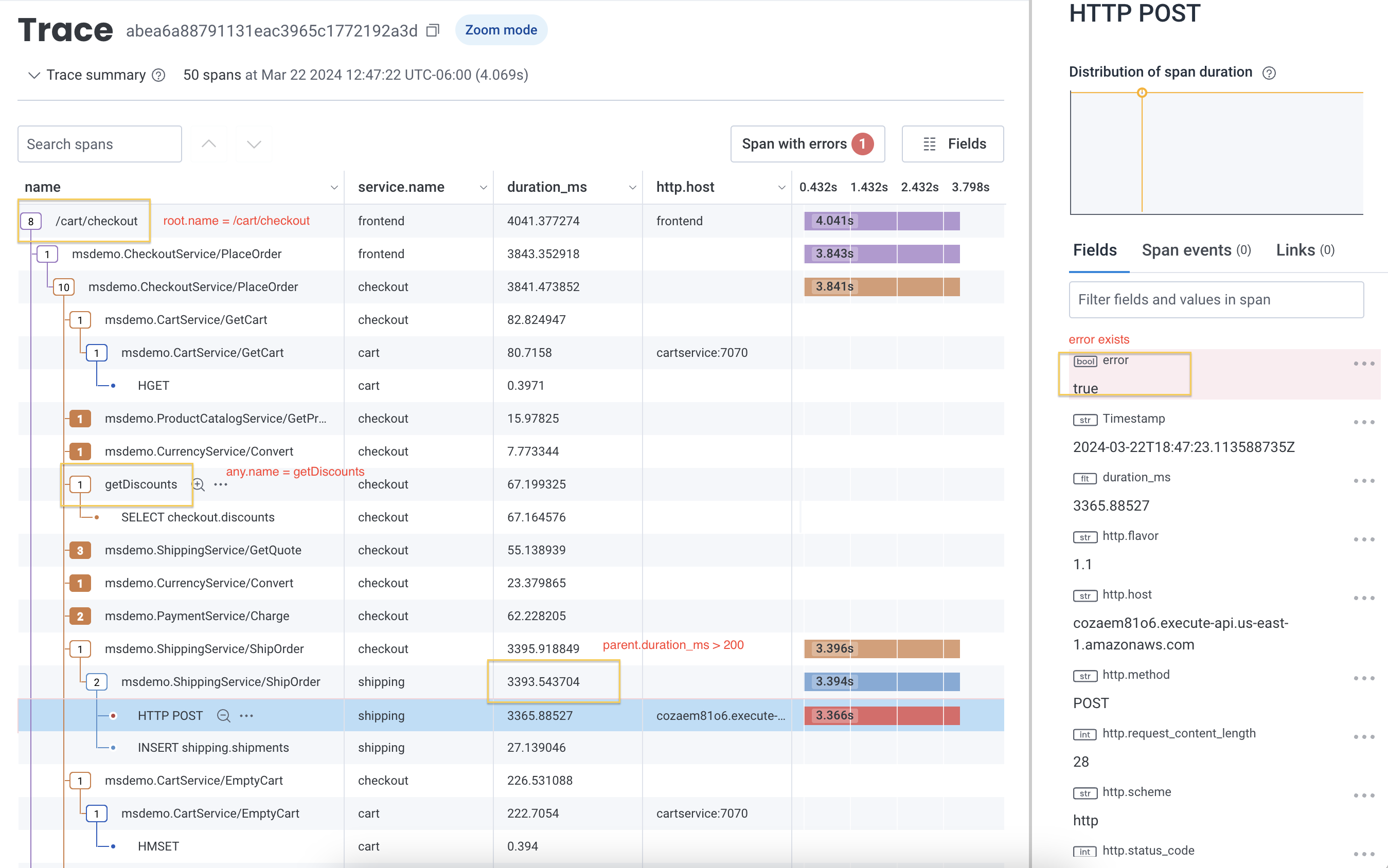 To explore more examples related to using relational fields with relational fields, visit [Examples: Query for Traces](/investigate/query/examples-traces/#relational-fields).
## Troubleshooting
Refer to [Common Issues with Queries](/troubleshoot/common-issues/queries/).
To explore more examples related to using relational fields with relational fields, visit [Examples: Query for Traces](/investigate/query/examples-traces/#relational-fields).
## Troubleshooting
Refer to [Common Issues with Queries](/troubleshoot/common-issues/queries/).